- Published on
A computational app for a proper evaluation of the irrigation effect over the aquifers
- Authors
Author
- Name
- Diego Sampietromail

Motivation
A correct design and control of the irrigation cycles is very important for the correct and efficient grow of crops. It is well known that a correct design of irrigation cycles increases its efficiency and reduces the amount of water required. An important objective in the agricultural industry is to design an optimal irrigation plan depending on crop requirements. The irrigation cycles have an effect on the quality and quantity of water. It becomes more relevant in areas of the world where water is scarce. Nowadays, several scientists are involved in different research projects that focus on finding alternative water sources for irrigation. One idea is to reuse human waste water [1]. This concept is based on the pollutant removal effect of the sun, the soil and the plants itself. However, it requires an important control of the polluted water evolution in the subsurface.
Numerical modelling is an important tool to help engineers and scientists design structures, simulate experiments, etc. In the context of this study, it can be used to design irrigation structures. It serves also to evaluate the propagation of pollutants or nutrients available in the irrigation water through the subsurface.
We present a useful app designed in Comsol that simulates the effects of different irrigation cycles on the soil saturation. It also can simulate the evolution of the pollutants dissolved in the water through the subsurface attending to its degradation. The application solves the Richard’s equation (eq 1) to obtain the groundwater flow field and its saturation.
The advection diffusion equation (eq 2) is used to simulate the transport of pollutants and nutrients.
The model is also prepared to evaluate the evolution of the dissolved elements involved in the organic matter degradation chain (figure 1).
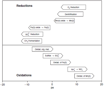
The chemical reactions considered in the model are the following:
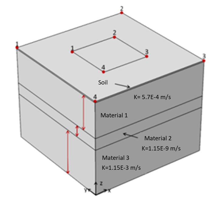
The app is fully parametrized. Regarding the geometry, it is up to the user to select the extension of the modelled area (Figure 2), the extension and location of the irrigation areas, etc. The app also considers different materials for the subsurface. Once the geometry is generated, the app allows the user to assign the properties of the materials such as the permeability or the porosity and introduce the irrigation planning which is read from an external file. Finally, the initial concentration of the different species is assigned together with the composition of the irrigation water.
The app is prepared to show several types of plots such as 2D slices that show the evolution of the saturation, the lead concentration, etc. It also shows the evolution of the groundwater level and water saturation at given observation points.
Example of application
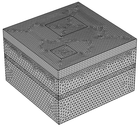
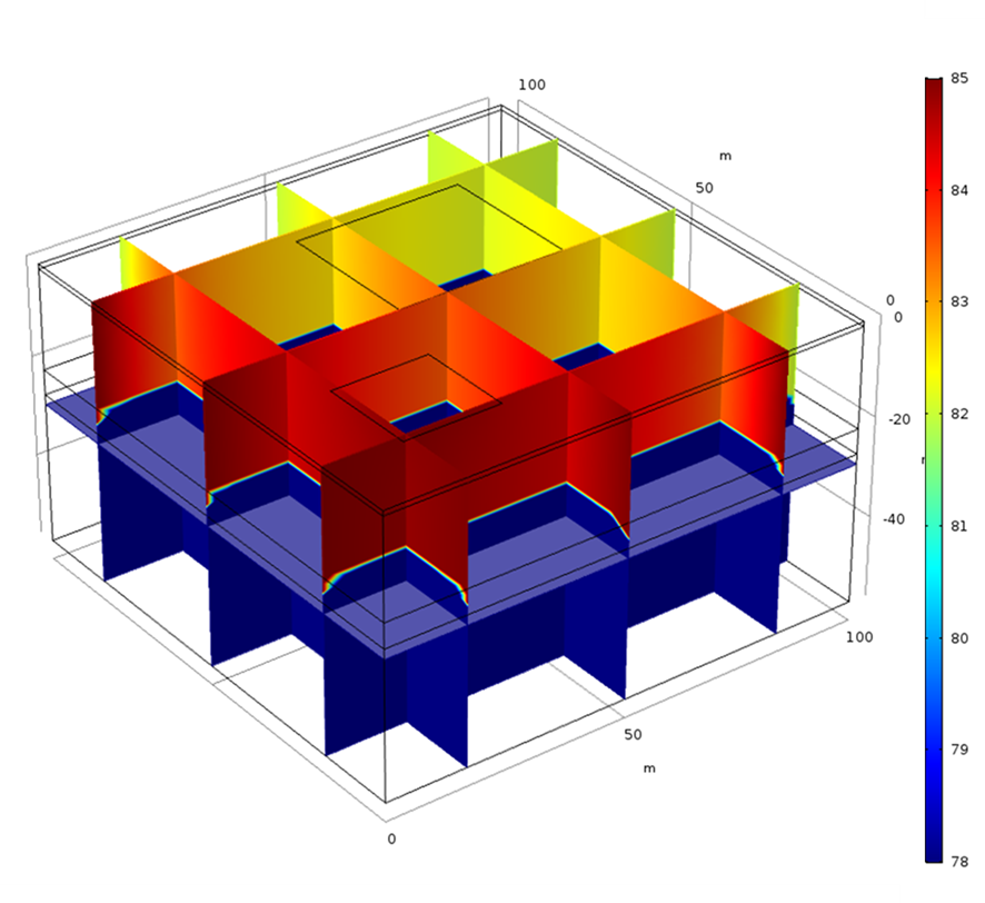
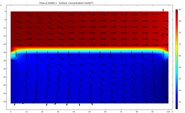
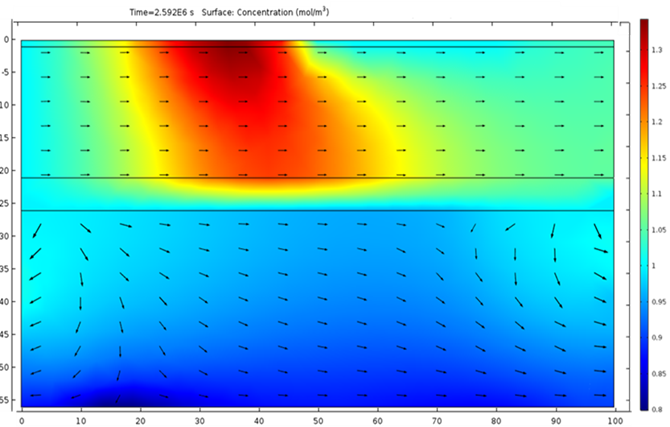
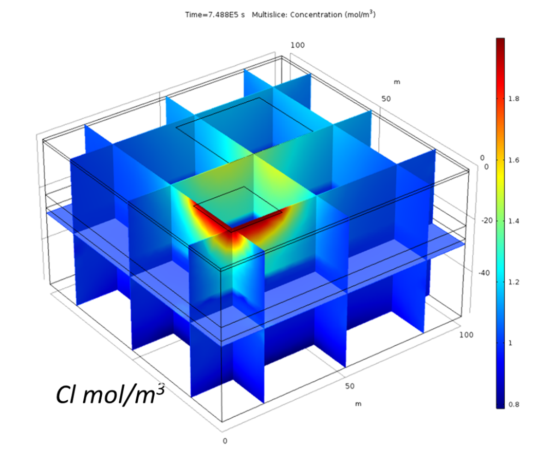
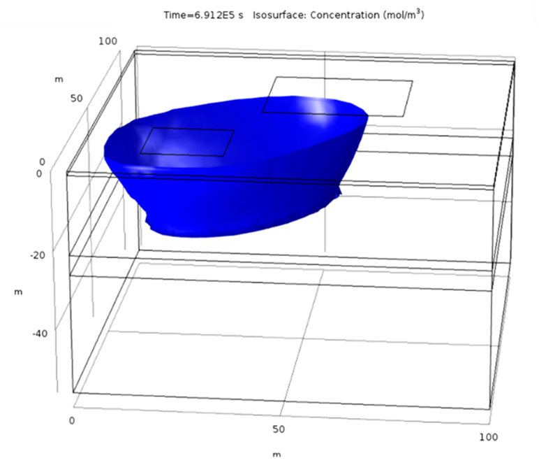
This example considers two permeable materials separated by a small aquitard. The hydraulic conductivity of the materials can be observed in Figure 2. Two irrigation zones are included (Figure 3). The model considers the irrigation of the small crop only. It considers a regional groundwater flow from south to north. Under these boundary conditions, the computed groundwater flow streams from the irrigation zone located south-west to the north north-east (Figure 4 and Figure 5). The groundwater level is higher in the upper aquifer than in the lower. There is a general flow from top to bottom through the aquitard. However, this flow between aquifers is small compared to the horizontal flow. This lower flow retards the movement of the concentration through the aquitard ( Figure 6). Figure 3 to 8 show different types of plots that can be used to visualize the results in the application. In addition, the app also contains different tables to export the results in a quantitative way.
The possibility of generated custom apps with Comsol allows the user to generate general models such as the one presented here that can be applied for different crops and areas.
References
[1] Hussain I.; L. Raschid; M. A. Hanjra; F. Marikar; W. van der Hoek. 2002. Wastewater use in agriculture: Review of impacts and methodological issues in valuing impacts. Working Paper 37. Colombo, Sri Lanka: International Water Management Institute.
[2] Appelo, C.A.J and Postma.D, 2014. Geochemistry, groundwater and pollution. 2nd edition.