- Published on
Computing groundwater age in Comsol Multiphysics: implementation of transient and steady-state methodologies
- Authors
Author
- Name
- Diego Sampietromail

Model description
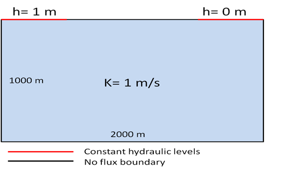
A simple 2D domain has been used to explore the methodology for implementing the water age calculation.
Figure 1 shows the geometry, parameters and boundary conditions of the example. It can be seen that groundwater will enter the domain by the upper left part (left red segment) and discharge through the upper right part (right red segment).
Mode 1: Transient simulation
Equation solved
For this model, a simple transport equation of an instant pulse of tracer (entering the domain) must be solved. Then, the equation that must be solved to computed groundwater age was proposed by Goode D.J.,1996:
Where A is the “Water age”, t is the time, C is the concentration of tracer and is the total duration of the tracer pulse.
Implementation in Comsol
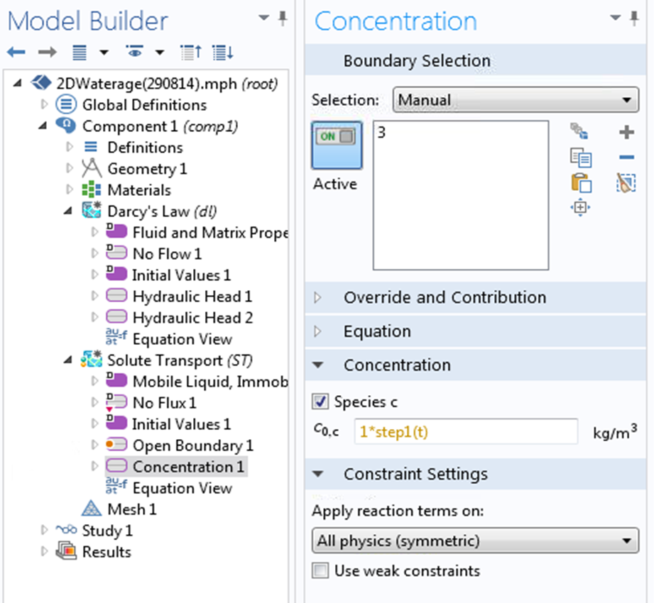
The transport boundary condition is a prescribed concentration on the recharge zone (hydraulic head=1), and open boundary in the discharge zone (hydraulic head=0). No flux is prescribed in the rest of the boundaries.
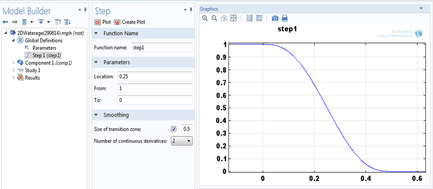
The required instant pulse of tracer was implemented by using the Comsol capability to create a time function associated to the boundary condition. This step function could be used as time function “step(t)” in the solute transport physics. A prescribed concentration boundary condition, associated to the time function “step(t)” was used to generate the pulse, as shown in Figure 2 and 3.
The model is then solved in a transient mode until all tracer concentration exits the model domain.
The time integration equation is implemented in the results section using the function timeint(from,to,variable) where from and to are t=0 and the time when all tracer exits the domain, respectively. In this case the expression needed is:
timeint(t0,T,c*t)/timeint(t0,T,c)
Where t0 and T is the initial and final time respectively for the integral and c is the solute concentration.
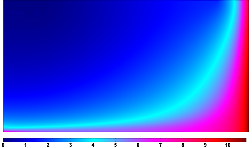
The result of use this expression is a surface showing the computed water age, as shown in Figure 4.
Mode 2: Steady state
Equation solved
The equation solved for steady state method is:
Where A is the water age (seconds), q is the Darcy flux (m/s), D is the dispersion tensor (m2/s), (Theta) is the porosity, ρ is the density (kg/m3) and F is the source term (equal to 0 in the conceptual model). In steady state the temporal term dA/dt is equal to 0.
Implementation in Comsol
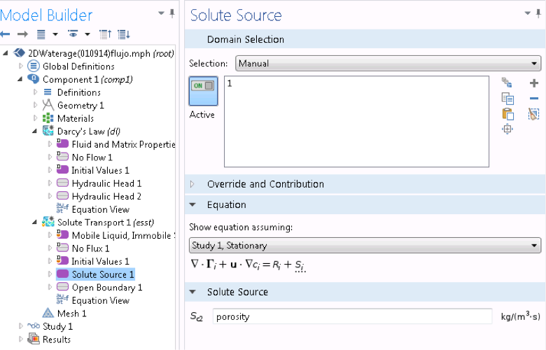
In this method the transport boundary conditions are open boundary for zones with prescribed hydraulic head and no flux for the rest of boundaries. Also a source term in all domain is needed to obtain the water age, the value of the source term is equal to one in the equation, if we use Darcy flux (q) and effective diffusion coefficient the source term must be the porosity, as shown in Figure 5.
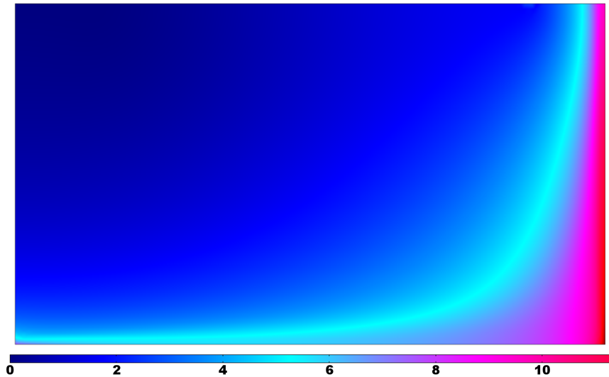
The computed water age is shown in Figure 6. It can be seen that computed results with the steady-state methodology is almost identical to what was computed at the transient approach (Figure 4).
Summary and conclusions
Two different approaches have been implemented in Comsol Multiphysics for calculating the water age in an aquifer. The steady-state methodology is easier, more accurate and much faster than the transient approach.
Acknowledgements
My more sincere thanks to Elena Abarca by her guidance and good advices and to Paolo Trinchero by his help to solve the steady state approach.
References
Goode D J, (1996). Direct simulation of groundwater age. Water resources research, vol 32.n No.12, pages 289-296