Introduction

PFLOTRAN is an open source subsurface flow and reactive transport code. It is capable of simulating many of the processes the affect flow and transport in porous media.

MARFA, on the other hand, is a code that simulates radionuclide transport in porous media. It uses a Monte Carlo algorithm to represent several processes, such as decay, longitudinal dispersion, diffusion into a rock matrix or equilibrium sorption. These processes are applied to particles, which represent packets of radionuclide mass. In the MARFA Static Path (MARFA-SP) version, transport is simulated in a fixed set of trajectories, with known parameters.

It is easy to see that some models can be computed in both PFLOTRAN and MARFA. While PFLOTRAN is more flexible, MARFA’s Monte Carlo algorithm is very efficient, due to it using solutions that have been precomputed and stored in lookup tables. Therefore, it would be interesting to compare the two codes. In this article, a model is run in both PFLOTRAN and MARFA, and its results and execution time are studied.

Model setup

The model is a simple straight fracture, with groundwater flow and a limited rock matrix on top. The size and parameters of this model are taken from (Iraola et al., 2019). The rock matrix could be modeled explicitly in PFLOTRAN by dividing the model in two sections. The bottom section would be the fracture and the top section would be the matrix. However, the performance is much better if we use PFLOTRAN’s multiple continuum capability. The multiple continuum method takes advantage of the fact that equations in the matrix are 1-dimensional to introduce several powerful optimizations.

Instant vs constant injections

In MARFA, (permanent) constant injection is not possible. The reason is that the code simulates particles until they reach the end of the model. If new particles were always released, there would never be a “final time”. Therefore, instant injection will be used. In other words, the source function will be a Dirac delta function centered at t=0.

\dot{m}_{in}\left(t\right)=m_{0}\delta(t)

Where $\dot{m}_{in}$ is the mass rate at the inlet and $m_0$ is the total mass that is injected in the model. For simplicity, we will set $m_0=1\ mol$ .

The same Dirac delta function could be applied to the PFLOTRAN model. However, PFLOTRAN shows high numerical dispersion for source functions with high discontinuities, such as the Dirac delta injection. Therefore, constant injection will be used for PFLOTRAN.

Although it may seem that this prevents comparison to the MARFA model, we can use the fact that the instantaneous mass breakthrough when using constant injection is proportional to the cumulative mass breakthrough when using Dirac delta injection. One way to see this is by using the solution from (Sudicky and Frind, 1982) for a fracture model with retention in finite matrix. In Laplace space, if we use a Dirac delta injection:

\bar{\dot{m}}_{Dirac}\left(s\right)=\bar{{\dot{m}}_{in}}\left(s\right)\bar{f_{ret}}\left(s\right)=m_0\bar{f_{ret}}\left(s\right)

Where $\bar{f_{ret}} \left(s\right)$ is the retention time function, $\bar{\dot{m}}_{Dirac}\left(s\right)$ is the breakthrough mass rate and $s$ is the Laplace variable. If we look at the cumulative breakthrough:

m\left(t\right)=\int_{0}^{t}{\dot{m}\left(\widetilde{t}\right)}d\widetilde{t}

An integral in Laplace space becomes a division by $s$ , so:

{\bar{m}}_{Dirac}\left(t\right)=\frac{\bar{{\dot{m}}_{in}}\left(s\right)}{s}=\frac{m_0}{s}\bar{f_{ret}}\left(s\right)

While, if we instead used a constant injection ${\dot{m}}_{in}\left(t\right)={\dot{m}}_0H(t)$ , where $H(t)$ is the Heaviside step function and {\dot{m}}_0 the mass rate at the inlet, the instantaneous breakthrough is:

{\bar{\dot{m}}}_{const}\left(s\right)=\bar{{\dot{m}}_{in}}\left(s\right)\cdot\bar{f_{ret}}\left(s\right)=\frac{{\dot{m}}_0}{s}\bar{f_{ret}}\left(s\right)

By comparing the two previous equations, we conclude that $m_{Dirac}$ and ${\dot{m}}_{const}$ are proportional to one another.

Low vs high velocity

In the model from (Iraola et al., 2019), groundwater velocity is set to $7.6\cdot{10}^{-7}\frac{m}{s}$ . Due to the relatively high velocity and the rest of parameters used in the model, matrix retention is relatively small. Therefore, another model will be run as well, using a velocity value of $7.6\cdot{10}^{-8}\frac{m}{s}$ , which is 10 times lower. The high velocity PFLOTRAN model was run up to 20 days in the paper. However, this is not sufficient for the low velocity case. In that case, the model was run up to 500 days. The timestep size was increased, in order to minimize the execution time.

Results

Execution time

Both codes were run in an Ubuntu version 20.04 virtual machine.

MARFA is not a parallel code; in other words, it always uses a single CPU. In order to compare the execution time, PFLOTRAN was run with only one CPU as well, so that the same amount of computational power is used in both codes.

PFLOTRAN took approximately 5 minutes and 15 seconds to compute the high velocity model, while 6 minutes and 19 seconds were required for the low velocity model. This contrasts with MARFA, which only took 22 seconds for the high velocity model and 8 seconds to run the low velocity model (run with 1 million particles). Therefore, MARFA computed the model about 14 times faster in the first case, and about 47 times faster in the second case! It might be possible to decrease the PFLOTRAN computation time by using less strict tolerances or timesteps, but the solution would be more numerically dispersive then.

Quality of the solution

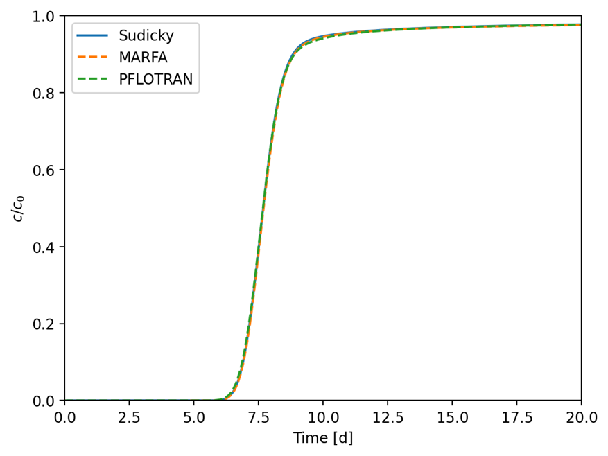
In both tests, MARFA and PFLOTRAN solutions are compared to the semianalytical solution by (Sudicky and Frind, 1982).

Figure 1 shows the MARFA and PFLOTRAN results in the high velocity case. Both codes agree very well with Sudicky’s solution.

**Figure 1**. Results for the high velocity case.

Results for the low velocity model are shown in Figure 2. There is now some early arrival in the PFLOTRAN solution, which is likely due to numerical dispersion. However, the quality of the solution is still very good in both codes.

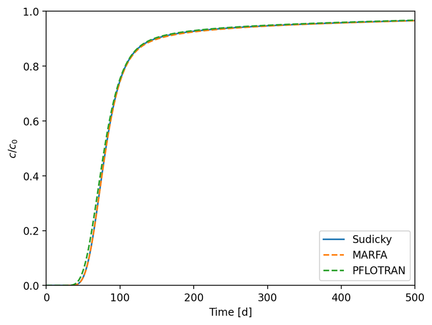
**Figure 2**. Results for the low velocity case.

In conclusion, both codes can be used to accurately simulate a simple fracture-matrix model, although MARFA-SP can compute the solution in significantly less time. On the other hand, note that the two codes are used quite differently: MARFA requires a set of trajectories with known advective time and transport resistance, while PFLOTRAN is applied to 3d models, with specified material properties and a velocity field.

References

Iraola, A., Trinchero, P., Karra, S., Molinero, J., 2019. Assessing dual continuum method for multicomponent reactive transport. Computers & Geosciences 130, 11–19. https://doi.org/10.1016/j.cageo.2019.05.007

Sudicky, E.A., Frind, E.O., 1982. Contaminant transport in fractured porous media: Analytical solutions for a system of parallel fractures*. Water Resources Research 18, 1634–1642. https://doi.org/10.1029/WR018i006p01634

How does MARFA compare to PFLOTRAN?

Author