Published on

Modelling Advection-Dispersion with Decay Chains

Authors

Author

  • Name
    Diego Sampietro
    mail

Motivation

Understanding the behaviour of pollutants in aquifers is a common issue we have to face as hydrogeologists. Numerical models are useful tools that allow us to predict the displacement and evolution of the pollutants in the subsurface. For this modelling task we usually use well-known software, but we find important keeping simple approaches in mind since they can be useful for learning about numerics insights and physics understanding.

To this end, we have developed a simple python program to compute the Advection-Diffusion equation (Bear, 1972) with first order decay and degradation chain [Eq.1] in 1 dimension using finite differences. This has been applied to simulate the nitrification chain, the degradation of ammonium generates nitrite and this specie when degrades produces nitrate. (NH4+NO2NO3NH_4^+ \rightarrow NO_2^- \rightarrow NO_3^-).

Description

The system modelled is represented by the following partial differential equations:

{NH4+t=D2NH4+x2x(aNH4+)λ1NH4+NO2t=D2NO2x2x(aNO2)+λ1NH4+λ2N02NO3t=D2NO3x2x(aNO3)+λ2N02λ3N03[Eq. 1]\tag*{[Eq. 1]} \begin{cases} \frac{\partial NH_4^+}{\partial t}=D\frac{\partial^2 NH_4^+}{\partial x^2}-\frac{\partial}{\partial x }(aNH_4^+)-\lambda_1 NH_4^+\\ \frac{\partial NO_2^-}{\partial t}=D\frac{\partial^2 NO_2^-}{\partial x^2}-\frac{\partial}{\partial x }(aNO_2^-)+\lambda_1 NH_4^+-\lambda_2 N0_2^-\\ \frac{\partial NO_3^-}{\partial t}=D\frac{\partial^2 NO_3^-}{\partial x^2}-\frac{\partial}{\partial x }(aNO_3^-)+\lambda_2 N0_2^--\lambda_3 N0_3^-\\ \end{cases}

Here, aa is the fluid velocity (water in the studied case) (m/s), DD is the diffusion coefficient (m2/sm^2/s) and λi\lambda_i is the half-time of the ii species where 1 refers to NH4+NH_4^+, 2 is NO2NO_2^- and 3 is NO3+NO_3^+.

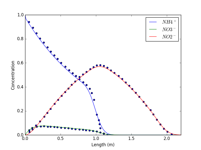
Obtained results (Figure 1) have been validated by comparing with the analytical solutions reported by (Cho et al. 1971).

Figure 1. Analytical solution from (Cho et al. 1971) (solid lines) vs numerical solution (dashed lines).

Numerical solution

Previous to the finite differences scheme development, it is useful to define some terms:

  • LL = Length of the domain.
  • NN = number of grid points.
  • x=L/N· x = L/N spatial discretization.
  • ii is the position at the domain being, therefore, ixi*· x where i[O,N1]i \in [O,N-1] is the real position.
  • TT = Total simulation time.
  • kk refers to a determined timestep being t· t= time step and ktk*·t the real time.

As can be seen in [Eq. 1] the proposed equation has a diffusive and a convective term. Using a Crank-Nicolson scheme for the diffusive term:

D2x2ui1k+1+(1t+Dx2)uik+1D2x2ui+1k+1=D2x2ui1k+(1tDx2)uik+D2x2ui+1k\frac{-D}{2· x^2}u^{k+1}_{i-1}+(\frac{1}{· t}+\frac{D}{· x^2})u_i^{k+1}-\frac{D}{2 · x^2}u^{k+1}_{i+1}=\frac{D}{2· x^2}u^{k}_{i-1}+(\frac{1}{· t}-\frac{D}{· x^2})u_i^{k}+\frac{D}{2 · x^2}u^{k}_{i+1}

Here, kk is the current time and ii is the cell in the domain.

And for the advection term:

auxa4x(Ui+1kUi1k+Ui+1k+1Ui+1k+1)\frac{\partial au}{\partial x} \approx \frac{a}{4· x}(U_{i+1}^k-U_{i-1}^k+U_{i+1}^{k+1}-U_{i+1}^{k+1})

Combining this two expressions, we obtain the advection diffussion equation in a cell point (i) at a time (k):

Uik+1Uikt=D2x2(Ui+1k2Uik+Ui1k+Ui+1k+12Uik+1+Ui1k+1)+a4x(Ui+1kUi1k+Ui+1k+1Ui1k+1)λUik\frac{U_i^{k+1}-U_i^k}{· t}=\frac{D}{2· x^2}(U_{i+1}^k-2U_i^k+U_{i-1}^k+U_{i+1}^{k+1}-2U_i^{k+1}+U_{i-1}^{k+1})+ \\ \frac{a}{4· x}(U_{i+1}^k-U_{i-1}^k+U_{i+1}^{k+1}-U_{i-1}^{k+1})-\lambda U_i^k

We define σ=Dt2x2\sigma = \frac{D· t}{2· x^2} and ρ=at4x\rho = \frac{a· t}{4 · x}. Reordering the previous approximation:

(σ+ρ)Ui1k+1+(1+2σ)ik+1(σ+ρ)i+1k+1=(σρ)Ui1k+(12σ)Uik+(σ+ρ)Ui+1k+t(λUik),i=1,..,N2.(-\sigma +\rho)U_{i-1}^{k+1}+(1+2\sigma)_i^{k+1}-(\sigma +\rho)_{i+1}^{k+1}=(\sigma -\rho)U_{i-1}^k+(1-2\sigma)U_i^k+(\sigma + \rho)U^k_{i+1}+· t (-\lambda U^k_i),\\ i=1,..,N-2.

This equation holds for all grid points containing in the domain i[1,N2]i\in [1,N-2]. The expression in the borders (0 and N-1) is given by the boundary conditions. In this case, we assume Neumann conditions in both boundaries.

The resulting expression for ii equal to 00 and N1N-1 is:

j=0:(1+σ+ρ)U0k+1(σ+ρ)Uik+1=(1σρ)U0k+(σ+ρ)Uik+1+tλ(U0k)j=0: (1+\sigma +\rho)U_0^{k+1}-(\sigma+\rho)U_i^{k+1}=(1-\sigma -\rho)U_0^{k}+(\sigma+\rho)U_i^{k+1}+· t \lambda(U_0^{k})
j=N1:(σ+ρ)UN2k+1+(1+σρ)UN1k+1=(+σρ)UN2k+(1σ+ρ)UN1k+tλ(UN1k)j=N-1: (-\sigma +\rho)U_{N-2}^{k+1}+(1+\sigma -\rho)U_{N-1}^{k+1}=(+\sigma -\rho)U_{N-2}^{k}+(1-\sigma +\rho)U_{N-1}^{k}+· t \lambda(U_{N-1}^{k})

The previous expression can be written as a linear system in matrix notation:

AUk+1=BUkfkAU^{k+1}=BU^{k}-f^k

Where:

A[NxN]=[1+σ+ρσ+ρ000000σρ1+2σσ+ρ000000σρ1+2σσ+ρ0000................................................0000σρ1+2σσ+ρ000000σρ1+2σσ+ρ000000σρ1+σρ]A[NxN]= \begin{bmatrix} 1+\sigma +\rho & -\sigma+\rho & 0 & 0 & 0 & 0 & 0 & 0\\ -\sigma-\rho & 1+2\sigma & -\sigma+\rho & 0 & 0 & 0 & 0 & 0\\ 0 & -\sigma-\rho & 1+2\sigma & -\sigma+\rho & 0 & 0 & 0 & 0\\ ... & ... & ... & ... & ... & ... & ... &...\\ ... & ... & ... & ... & ... & ... & ... & ...\\ 0 & 0 & 0 & 0 & -\sigma-\rho & 1+2\sigma & -\sigma+\rho &0\\ 0 & 0 & 0& 0 & 0 & -\sigma-\rho& 1+2\sigma& -\sigma+\rho \\ 0 & 0 & 0 & 0 & 0 & 0 & -\sigma-\rho & 1+\sigma-\rho \end{bmatrix}
B[NxN]=[1σρσρ000000σ+ρ12σσρ000000σ+ρ12σσρ0000................................................0000σ+ρ12σσρ000000σ+ρ12σσρ000000σ+ρ1σ+ρ]B[NxN]= \begin{bmatrix} 1-\sigma -\rho & \sigma-\rho & 0 & 0 & 0 & 0 & 0 & 0\\ \sigma+\rho & 1-2\sigma & \sigma-\rho & 0 & 0 & 0 & 0 & 0\\ 0 & \sigma+\rho& 1-2\sigma & \sigma-\rho & 0 & 0 & 0 & 0\\ ... & ... & ... & ...& ... & ... & ... & ...\\ ...& ... & ...& ... &... & ... & ... & ...\\ 0 & 0 & 0 & 0 & \sigma+\rho & 1-2\sigma & \sigma-\rho &0\\ 0 & 0 & 0& 0 & 0 & \sigma+\rho & 1-2\sigma& \sigma-\rho\\ 0 & 0 & 0 & 0 & 0 & 0 & \sigma+\rho & 1-\sigma+\rho \end{bmatrix}

Uk+1U^{k+1} and UkU^k are the solution at a given time k and k+1.

ff is the source term which in our case is a vector of length NN with the following expression:

f[N]=Uk[tλ,tλ,....,tλ]f[N]= U^k\begin{bmatrix} -· t \lambda ,-· t \lambda,....,-· t \lambda \end{bmatrix}

Conclusions

The proposed numerical scheme and its implementation are able to reproduce the results of the analytical solution reported by (Cho et al. 1971). The model describes the dissolved species movement through advection, diffusion and takes into account the degradation by first order decay.

References

  • Cho C. M., 1971. Convective transport of ammonium with nitrification in soil.Canadian journal of soil science.
  • Bear J., 1972. Fluid dynamics in porous media.