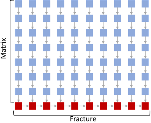
On June 2021, the new version of iCP (v 2.0) was released. One of the several improvements and capabilities included in this version is the possibility to add extra dimensions to your reactive transport models. Extra dimensions extend a standard geometry with additional spatial dimensions and they make it possible to solve PDEs in any number of independent variables, beyond 3D and time. For fracture-matrix systems, the extra dimension approach included in iCP allows to account for matrix diffusion mechanisms with their geochemical implications without having to represent the matrix explicitly in the finite element mesh. This approach simulates the movement of chemical species trough the fractures and diffusion through the matrix by representing the low permeable matrix as a set of individual 1D elements (lines) connected to the nodes of the fracture (Figure 1).

The developments carried out in the iCP code allow to include chemical reactions in both domains, the extra dimension representing the matrix and the fracture. The main benefit of this methodology is the possibility to include matrix diffusion in discrete fracture networks (DFNs) of thousands of fractures with complex intersections where it can be challenging or impossible to mesh the fractures and rock matrix. In this context, the extra dimensions of COMSOL can be very handy when the matrix has low permeability and transport is diffusion dominated.

This post shows an example of these capabilities.

Model description

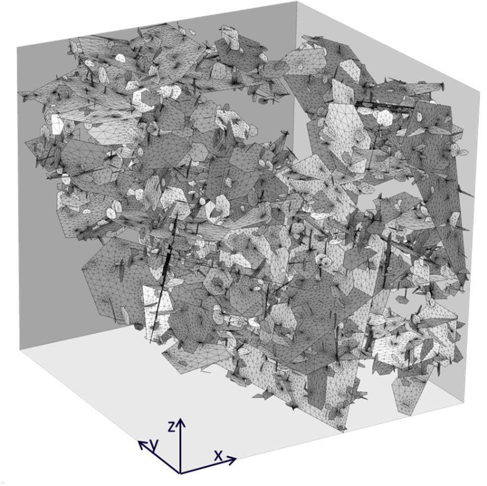
A 3D fractured carbonated media formed by calcite with a constant circulation of groundwater that contains magnesium chloride is considered. In this system, magnesium-rich groundwater flows through the fractures leading to calcite dissolution and eventually dolomite formation. The fracture system is based on a discrete fracture network (DFN) formed by 3,531 hexagonal fractures inside a cube of 200 meters of length centered at origin (Figure 2). The hydraulic properties of the fractures (hydraulic conductivity, aperture and storativity) are spatially heterogeneous.

The chemical composition for the initial and boundary waters considered is illustrated in Table 1. The matrix is assumed to initially contain 2 x10^-4 moles/kg_medium of calcite. In this system, transport is dominated by advection through the fractures. The travel time to through the materials is large enough to assume local chemical equilibria and hence the dissolution/precipitation of calcite and dolomite is assumed to occur in equilibrium.

Due to the complexity of the fracture network, the matrix cannot be modelled explicitly, and then it is represented as an extra-dimension by considering a characteristic length of 1 m with one finite element (two nodes). Thus, each node of the fracture is connected to a linear element of the extra dimension according to the scheme of the Figure 1. Regarding the boundary conditions, a prescribed hydraulic head (Dirichlet boundary condition) is imposed along the fractures of the east boundary (h = 1 m) and at the west boundary (h = 0 m). The rest of boundaries are assumed as no flow of both solute and water. The groundwater flow is solved to reach the steady state solution. The reactive transport simulation covers a total simulation time of 210 years.

Results

Numerical results from the flow simulation show a groundwater gradient from east to west which is focalized on two preferential paths: one in the upper northern part and the other in the lower Southern part (Figure 3). These paths are mainly controlled by the largest and most connected structures. The rest of the fractures present lower flow velocities because they have small transmissivities, they are not well-connected or are even disconnected with the two main set of fractures.

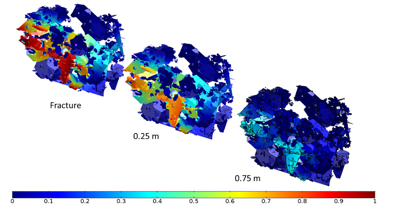
Figure 3 shows the concentration of chloride in the fracture-matrix system. Numerical results also show the presence of two preferential paths for solute transport. Thus, at the end of the simulation the chloride-magnesium plume spreads mainly along the upper north part and at the bottom. Also, after 200 years of simulation, the chloride concentration in the matrix at 0.75 meters form the fractures is lower than half of the concentration entering through the boundary (Figure 4), indicating a strong retardation effect of matrix diffusion processes.

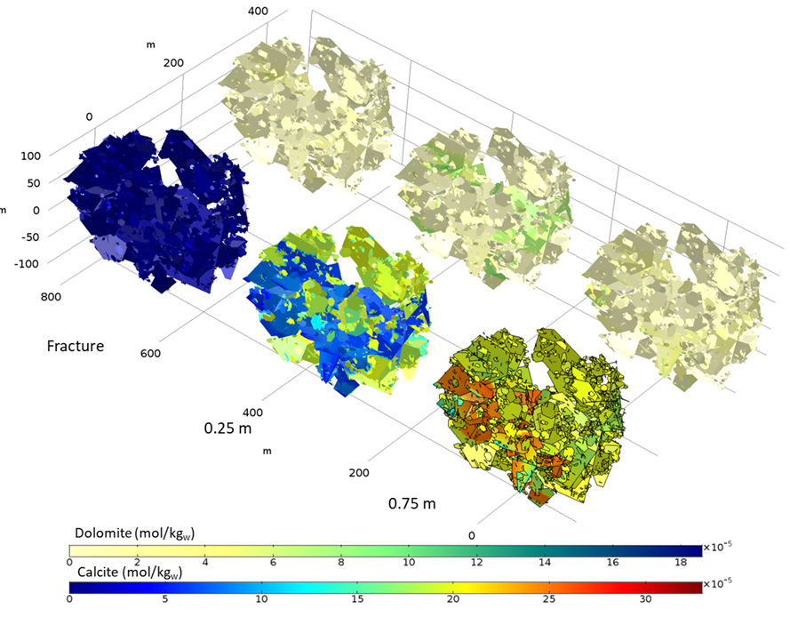
Reactive transport results show the progressive replacement of calcite by dolomite due to the movement of the enriched chloride-magnesium plume (Figure 5 and Figure 6). Although the incoming water is initially undersaturated in dolomite, the mixing between the boundary water and the initial water in the matrix leads to oversaturation of this mineral at the front of the magnesium-rich plume. Note that dolomite precipitation occurs mainly at a distance of 0.25 m from the contact between matrix and fractures, and only a small amount of dolomite precipitates along the fractures (Figure 5). Numerical results also demonstrated that in some areas once calcite is depleted, mixing induces the dissolution of dolomite.

Summary and conclusions

This example introduces one of the newest capabilities of iCP, the use of extra dimensions. The results show how iCP can deal with complex discrete fracture networks while accounting for the effect of the rock matrix, which is included as an extra dimension. This setup accounts for the diffusion of chemical species from the fractures to the matrix and vice versa and the diffusion of chemical species through the matrix considering geochemical reactions. This example shows that the use of extra dimension is an efficient way to include matrix diffusion processes in complex geometries including DFNs with thousands of fractures. It should be noted, however, that the extra dimension approach can be applied only when the permeability of the matrix is very low and transport is governed by diffusion.

If you want to know more about the new capabilities of iCP, you can check out this post.