- Published on
Ogata and Banks Analytical Solution
- Authors
Author
- Name
- Albert Nardimail

Background
Numerical modelling is nowadays the reference tool to simulate and predict the behaviour of hydrogeological systems. This fact, however, has not stopped the research and the continuous development of analytical solutions for the different porous media equations. Analytical solutions are still useful tools today for system understanding and fast prediction scenarios.
At Amphos21, we also use analytical solutions to verify code developments. They are valuable resources to validate numerical implementations and explore the numerical method limits for handling certain physics (for example advection predominant problems when using FEM).
In the last years, we have been involved in the development of different reactive transport codes. For their verification, we have been using intensively the analyitical solution Differential Equation of Longitudinal Dispersion in Porous Media provided by Akio Ogata and R. B. Banks (1961). This solution does not involve chemical reactions, we use it mainly to verify that the conservative tracers are handled correctly. This way we have fast feedback to determine if possible differences in reactive species are caused or not by errors or wrong settings in the solute transport equation resolution.
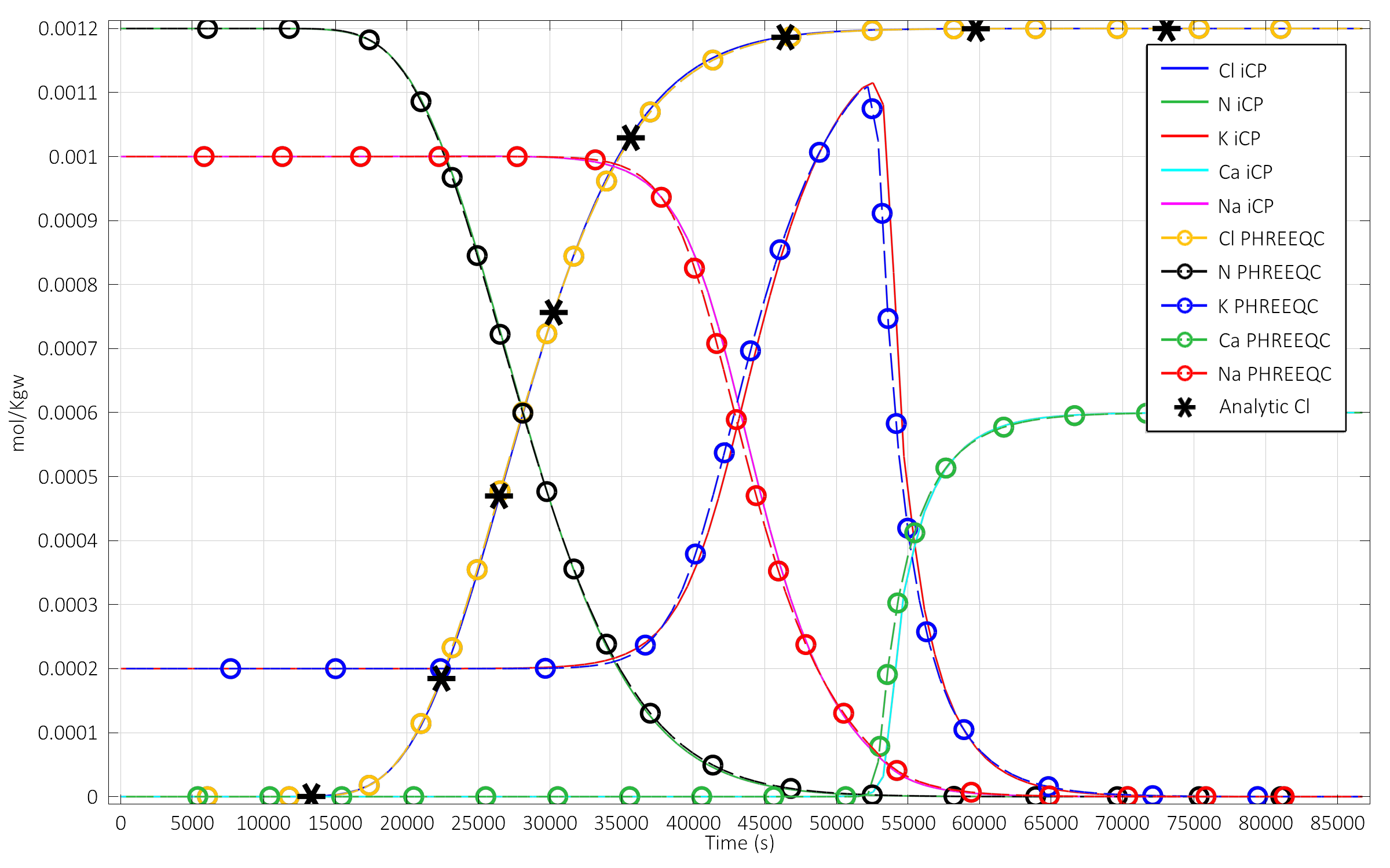
See this use on one of the iCP verification problems (Figure 1). The chloride, which is a conservative species in this case, fits to the analytical solution.
Ogata and Banks 1961
Ogata and Banks analytical solution dates from 1961 and can be found in the following USGS report.
It solves the ADE equation for a Continuous Source of Infinite Duration and a 1D domain:
with the following boundary and initial conditions:
where is the concentration , is the distance , is the retardation factor , the effective dispersion/difusion , the flow velocity and the concentration at the upstream boundary .
The analytical solution is:
Experiment
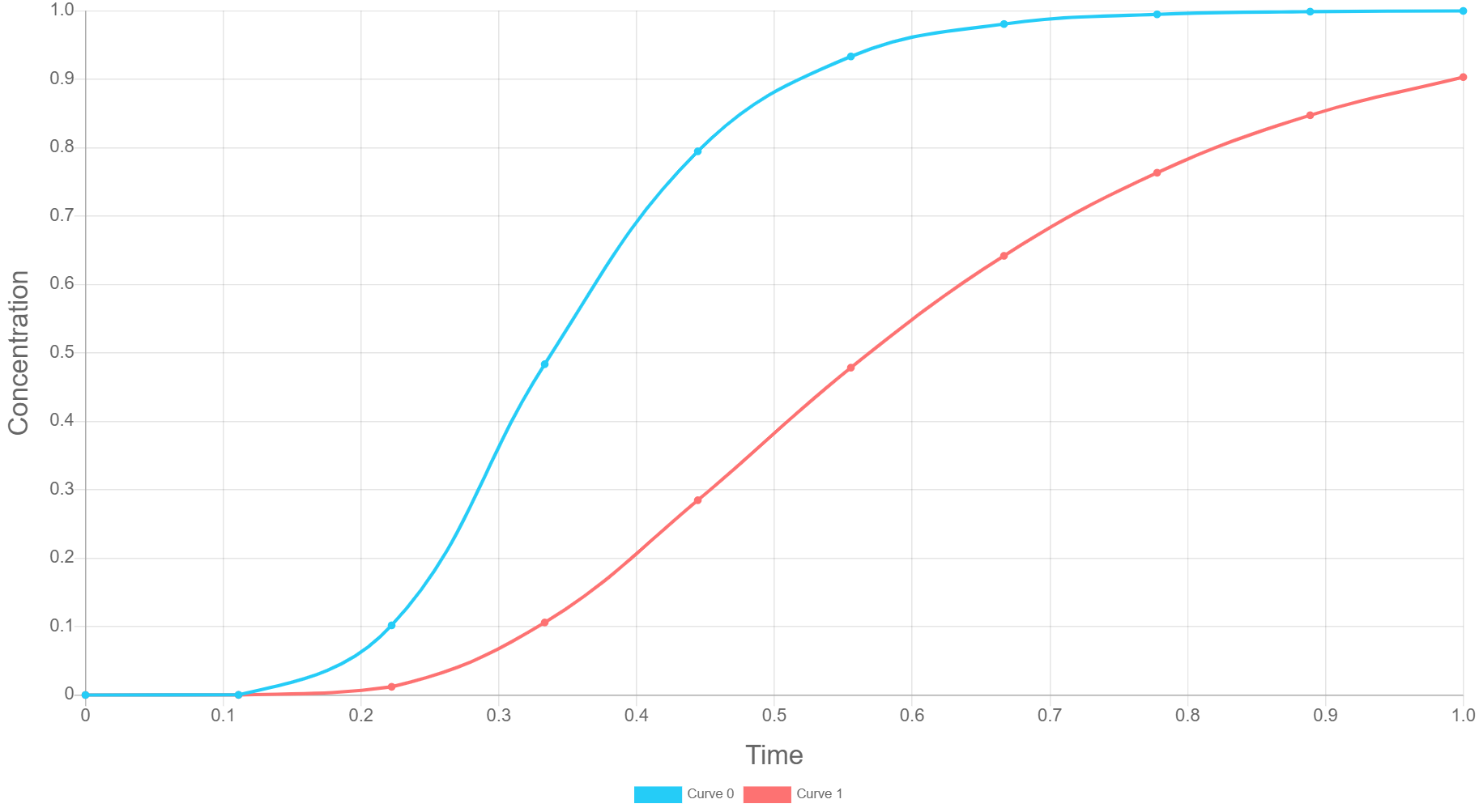
We have implemented the Ogata and Banks solution in a web application to predict quickly the arrival concentrations at a distance . We use it to have first estimations of tracer arrival times and the role that play different parameters on modifying the arrival curve shape.
Just set your simulation parameters and play Add Curve to get your results. We hope you enjoyed it!
References
Ogata, A., & Banks, R. B. (1961). A solution of the differential equation of longitudinal dispersion in porous media: fluid movement in earth materials. US Government Printing Office.